Introduction
Fractals have fascinated mathematicians and artists for decades. They are infinitely complex patterns generated by simple iterative rules. Most people are familiar with the 2D Mandelbrot set, but its 3D counterpart, the Mandelbulb, offers a stunning and intricate world to explore. Unlike traditional polygonal 3D models, fractals are procedural, meaning their geometry is defined mathematically rather than with vertices.
In this post, we’ll explore how to render the Mandelbulb in WebGL using ray marching. This approach allows us to calculate each pixel on the fly by tracing rays through space and determining where they intersect the fractal. Along the way, we’ll cover:
- The mathematics and iteration formula behind the Mandelbulb.
- Distance estimation and how it drives efficient ray marching.
- Orbit traps for fractal coloring.
- Soft shadows, surface normals, and depth of field.
- Physically based shading with diffuse, specular, and Fresnel terms.
- Progressive frame accumulation for smoother, refined images.
How Mandelbulbs appear in film and visual effects.
By the end, you’ll understand both the theory and practical shader implementation behind a fully interactive Mandelbulb viewer like the one demonstrated below. Take a minute to play around with the demo. Click and drag to interact with the geometry, and experiment with the parameters to explore different configurations of the fractal.
The Mandelbulb fractal
The Mandelbulb was first proposed in 2009 by Daniel White and Paul Nylander as a 3D analogue to the famous 2D Mandelbrot set. While the Mandelbrot set exists in the complex plane, the Mandelbulb uses 3D Cartesian coordinates converted to spherical coordinates to achieve the same kind of self-similar, infinitely complex structure in three dimensions.
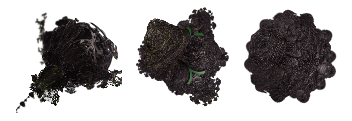
Visually, the Mandelbulb exhibits elaborate, bulbous structures with spiraling filaments and intricate cavities. Depending on the power parameter and bailout, the shape can vary from smooth, almost organic forms to chaotic, spiky structures.
Rendering these fractals in real-time is challenging because they are not stored as meshes. You must compute their geometry procedurally, which is where ray marching and distance estimation come into play.
Key characteristics
- Fractal iteration: Points in space are iteratively transformed by a mathematical formula.
- Power Parameter: Controls the “twistiness” and overall complexity of the fractal. Higher powers create more elaborate structures.
- Bailout Radius: Determines when a point is considered to have “escaped” the fractal, similar to the 2D Mandelbrot set.
The mathematical formula
To generate the Mandelbulb, we perform the following steps for a point \(\mathbf{p} = (x, y, z)\)
Step 1: Convert Cartesian coordinates to spherical coordinates:
\[r = \sqrt{x^2 + y^2 + z^2}, \quad \theta = \arccos\left(\frac{z}{r}\right), \quad \phi = \arctan2(y, x)\]Step 2: Raise the radius and angles to the desired power:
\[r \gets r^{\text{power}}, \quad \theta \gets \theta \cdot \text{power}, \quad \phi \gets \phi \cdot \text{power}\]Step 3: Convert back to Cartesian coordinates:
\[\mathbf{z} = r \begin{bmatrix} \sin \theta \cos \phi \\ \sin \theta \sin \phi \\ \cos \theta \end{bmatrix} + \mathbf{p}_0\]Step 4: Repeat this iteration up to a maximum number of iterations or until the
distance from the origin exceeds the bailout radius.
Distance estimation
To render the Mandelbulb efficiently, we use a distance estimator (DE), which tells us the approximate distance from any point in space to the fractal’s surface. This allows ray marching to take safe, large steps toward the surface. Additionally, orbit traps are often used for coloring, giving interesting patterns depending on how the ray orbits the fractal during iteration.
The DE uses the accumulated derivative \(\mathbf{𝑑r}\) to compute the approximate distance to the fractal’s surface:
\[d \approx 0.5 \frac{\log r \cdot r}{dr}\]Where:
- \(r = \|\mathbf{z}\|\) at the final iteration.
\(dr\) is updated each iteration as:
\[dr \gets r^\text{power} \cdot \text{power} \cdot dr + 1\]
This is how the distance estimator is implemented.
// Structure to store distance estimate output
struct DEOutput {
    float dist; // Distance to Mandelbulb surface
    float iter; // Iterations taken
};

// Distance Estimator
DEOutput mandelbulbDE(vec3 pos) {
    vec3 z = pos;           // Initialize z to the point we're evaluating
    float dr = 1.0;         // Derivative term for distance estimate
    float r = length(z);    // Distance from origin
    int it = 0;             // Iteration counter

    for(int i = 0; i < 1000; i++) {  // Hard-coded loop limit (GLSL needs const)
        if(i >= iterations) break;   // Stop if max iterations reached
        r = length(z);               // Current distance from origin
        if(r > bailout) break;       // Escaped fractal radius

        // Convert to spherical coordinates
        float invr = max(r, 1e-6);   // Avoid division by zero
        float theta = acos(clamp(z.z / invr, -1.0, 1.0));
        float phi = atan(z.y, z.x);

        // Scale radius and angles by power
        float zr = safePow(r, power);
        theta *= power;
        phi *= power;

        // Convert back to Cartesian coordinates
        z = zr * vec3(sin(theta) * cos(phi), sin(theta) * sin(phi), cos(theta)) + pos;

        // Update derivative for distance estimation
        dr = zr * power * dr + 1.0;
        it++;
    }

    r = max(length(z), 1e-6); // Avoid log(0)
    float dist = clamp(0.5 * log(r) * r / dr, 0.000001, 1000.0);
    return DEOutput(dist, float(it));
}
Ray marching
At the heart of rendering fractals like the Mandelbulb lies ray marching (also known as sphere tracing). Unlike rasterization, where geometry is explicitly defined by meshes, ray marching works directly with an implicit surface described by a mathematical function, in this case, the Mandelbulb’s distance estimator (DE).
Ray marching is a technique where we shoot rays from the camera into the scene and repeatedly march along them, guided by the distance estimator.
The DE tells us the minimum distance from a given point in space to the nearest surface. By taking steps of this length, the ray avoids overshooting and converges toward the fractal surface.
Here’s the GLSL code that implements ray marching:
float t = 0.0;        // Distance traveled along the ray
bool hit = false;     // Flag to record if we hit the fractal
vec3 p;               // Current point on the ray

// Main ray marching loop
for(int i = 0; i < MARCH_CAP; i++) {
    if(i >= maxSteps) break;        // Respect user-defined step limit
    p = ro + rd * t;                // Compute current position along ray
    DEOutput res = mandelbulbDE(p); // Evaluate distance estimator
    float d = res.dist;             // Distance to nearest surface

    if(d < EPS_H) {   // If we're closer than the hit threshold
        hit = true;   // We consider it a surface hit
        break;        // Exit loop early
    }

    t += d;              // Advance ray forward by safe step
    if(t > FAR_T) break; // Stop if ray leaves the scene bounds
}
| Symbol | Meaning |
|---|---|
ro | Ray origin (camera position, possibly shifted for depth of field) |
rd | Normalized ray direction |
t | Distance traveled along the ray |
d | Distance to the nearest surface, returned by the distance estimator |
The loop accumulates t until one of three conditions is met:
- The ray is close enough to the fractal,
d < EPS_H: Hit detected. - The ray exceeds the scene’s bounds,
t > FAR_T: Escaped. - The step limit (maxSteps) is reached: Give up.
The beauty of sphere tracing lies in its efficiency. It marches in large steps in empty space because the DE guarantees no surface exists within d. It marches in small steps near the surface allowing precise convergence. This adaptive stepping makes raymarching ideal for fractals, which combine vast voids with extreme detail.
After the loop, there are two possible outcomes:
- If a hit is found, the shader shades the surface using normals, shadows, and physically based rendering (PBR).
- If the ray misses, the pixel remains the background color (black in this shader).
This binary hit / miss logic is what turns pure math into a rendered 3D fractal.
Orbit traps
Orbit traps use simple geometric “traps” to record how a point’s orbit behaves while iterating on the geometry. During the distance-estimation loop, we track the minimum distance to a chosen trap shape. This single scalar, often called the trap value, becomes a rich signal for artistic coloring.
Each iteration updates z = f(z) + pos. While iterating, we compute a trap distance from z to a shape (plane, sphere shell, axis, cube). We keep the minimum encountered value:
- If the orbit repeatedly skirts a trap, the minimum distance becomes small.
- If it never comes close, the value remains larger.
- This variation across space produces smooth, detail-revealing colors.
The demo supports a sample set of orbit traps: Plane, Sphere, Axis, Cube. Their implementation is surprisingly simple.
// Computes a scalar trap signal from the current iterate z
float trapDistance(vec3 z) {
    float trap = 0.0;
    if      (trapMode == 0) trap = abs(z.y);             // Plane trap (Y=0)
    else if (trapMode == 1) trap = abs(length(z) - 1.0); // Spherical shell (r=1)
    else if (trapMode == 2) trap = length(z.xy);         // Axis trap (distance to Z axis)
    else if (trapMode == 3) trap = max(max(abs(z.x), abs(z.y)), abs(z.z)); // Cube trap
    return trap;
}
And here is how we integrate this logic into the distance estimator:
// Structure to store distance estimate output
struct DEOutput {
    [...]
    float trap; // Orbit trap value
};

DEOutput mandelbulbDE(vec3 pos) {
    [...]
    float trap = 1e6;     // Start large; we take mins over iterations

    for (int i = 0; i < 1000; i++) {
        if (i >= iterations) break;

        r = length(z);
        trap = min(trap, trapDistance(z)); // Update orbit trap signal
        if (r > bailout) break;
    }

    [...]
}
Soft shadows
We already have a distance estimator (DE) for the Mandelbulb. That same DE lets us query how close geometry is along a shadow ray. Instead of a hard yes / no occlusion test, we accumulate a penumbra factor that fades smoothly to black when nearby surfaces skim the shadow ray.
Let’s introduce the parameters the shadow calculation uses:
| Parameter | Meaning |
|---|---|
ro | Origin of the shadow ray, usually the shaded point offset slightly along the surface normal to avoid self-shadowing. |
rd | Direction of the shadow ray, pointing toward the light (normalized). |
mint | Near starting distance along the ray (often 0.0 or a small epsilon). |
maxt | Maximum marching distance. For directional lights: a large scene far plane; for point lights: distance to the light (length(lightPos - ro)). |
maxSteps | Upper limit on how many marching iterations are performed. Prevents infinite loops and controls performance. |
k | Shadow hardness factor. Larger k produces sharper, harder shadow edges; smaller k makes softer penumbras. |
To evaluate if a point is fully or partially occluded, we need a heuristic. Each step samples the DE at p = ro + rd * t. The SDF distance h = mandelbulbDE(p).dist determines how far we are until we’d hit geometry if we marched from p. The ratio h / t approximates the angular clearance between the ray and the nearest surface, i.e., how close geometry comes to grazing the light ray. Smaller means tighter occlusion.
res = min(res, k * h / t) keeps track of the minimum (worst) clearance encountered so far. The scale factor k controls the edge hardness, with k = 16.0 being a good default. A range of 8-32 is reasonable. The exact value would depend on how crisp we want the shadow edge to be.
- Higher k means sharper, more binary edges.
- Lower k means blurrier, softer penumbras.
If we ever get h < EPS_H, we’re effectively inside geometry along the shadow ray which means that the point is fully in shadow (return 0).
Pure sphere tracing would step by h. On fractals, DE can vary wildly. Clamping with t += clamp(h, 0.01, 0.5) avoids overstepping thin filaments which would cause light leaks / banding, and keeps step cadence stable enough for a smooth res curve.
The shadow value is used as a multiplier to the direct light term with: NdotL *= shadow;.
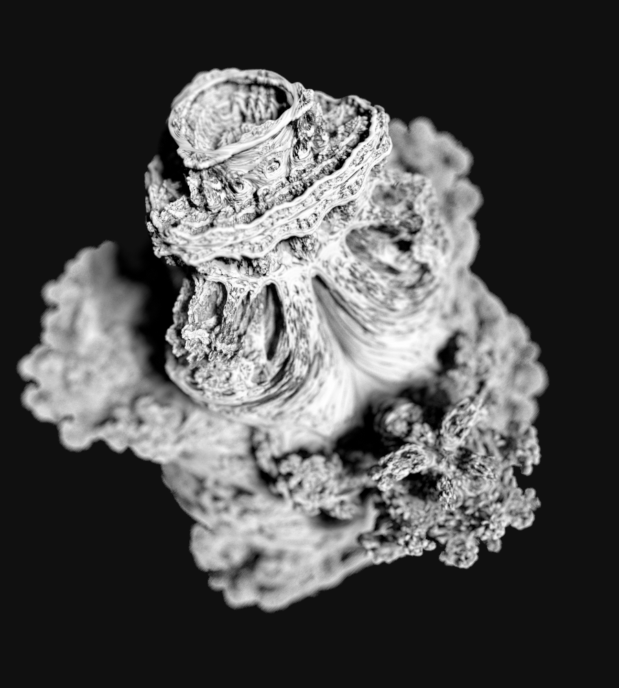
Visualization of the shadowing term
Solving shadowing issues
Even with a solid soft-shadow implementation, certain artifacts tend to show up when ray-marching complex fractals. These issues aren’t bugs so much as numerical side effects of distance estimation and limited marching precision. The good news is that each has well-known remedies.
| Issue | Remedy |
|---|---|
| Self-shadow acne | A bias is added to the ray origin along the surface normal, e.g.: softShadow(p + n * (2.0 * EPS_H), l, 0.0, FAR_T, 64). |
| Peter-panning (detached shadows) | If shadow edges look lifted or floating, reducing the bias or slightly increasing k hardens the edge. |
| Banding in penumbra | Caused by large step jumps, and mitigated by clamp(h, 0.01, 0.5). |
Here’s the implementation:
// Soft shadow via sphere tracing
// Casts a shadow ray from a shaded point toward the light, and
// attenuates lighting smoothly when geometry comes close to the ray.
// Instead of a binary hit/miss, it builds a soft penumbra factor.
float softShadow(vec3 ro, vec3 rd, float mint, float maxt, int maxSteps) {
    // ro   : ray origin (usually surface point + normal bias)
    // rd   : ray direction (toward light, normalized)
    // mint : near starting distance along the ray
    // maxt : maximum distance to march (far plane or distance to light)
    // maxSteps : maximum number of iterations allowed

    float t = mint;      // current parametric distance along the ray
    float res = 1.0;     // shadow factor, starts fully lit (1.0 = no shadow)

    // k controls how sharp the shadow edges appear.
    // Larger values -> harder shadows; smaller values -> softer penumbra.
    const float k = 16.0;

    // Fixed iteration cap of 128 to satisfy GLSL loop unrolling rules.
    for(int i = 0; i < 128; i++) {
        // Bail out if we’ve already taken the requested number of steps,
        // or if we’ve marched beyond the maximum allowed distance.
        if(i >= maxSteps || t > maxt)
            break;

        // Sample the signed distance field at the current point
        float h = distAt(ro + rd * t).dist;

        // If we’re closer than the hit epsilon, the ray intersects geometry
        // → fully occluded (hard shadow, no light passes through).
        if(h < EPS_H)
            return 0.0;

        // Update shadow factor: ratio h/t estimates angular clearance
        // between the ray and the nearest surface.
        // Take the minimum over all steps → worst-case occlusion.
        res = min(res, k * h / t);

        // Sphere trace step: advance along the ray by 'h'.
        // To avoid visual artifacts, clamp the step:
        //   - at least 0.01 (prevents infinite tiny steps near surface noise)
        //   - at most 0.5 (prevents huge leaps that skip thin geometry).
        t += clamp(h, 0.01, 0.5);
    }

    // Clamp result to [0,1] just in case numerical errors push it outside.
    return clamp(res, 0.0, 1.0);
}
and this is how it’s used:
// bias to avoid self-shadowing acne
float shadowBias = 2.0 * EPS_H;
float sh = softShadow(p + n * shadowBias, l, 0.0, FAR_T, 64);
Surface normals
To shade the Mandelbulb with lighting, we need a surface normal at every hit point. Unlike triangle meshes, there are no explicit surface normals in a fractal SDF, and as such, we have to approximate them numerically. The key idea is to use the gradient of the signed distance function. In math terms:
\[\mathbf{n} = \nabla d(\mathbf{p})\]where d(p) is the distance estimator. In practice, we evaluate the DE at points around p and combine them.
Tetrahedron sampling pattern
Instead of naïve central differences on the X, Y, and Z axes, this code uses a tetrahedral sampling pattern:
- Four offset vectors (
k1..k4) that are evenly distributed around the point. - We sample the distance at each offset:
d1..d4. - Then recombine into a gradient approximation:
n ≈ normalize(k1*d1 + k2*d2 + k3*d3 + k4*d4).
This approach:
- Uses only 4 DE calls instead of 6 (cheaper).
- Produces smoother, less axis-aligned normals (reduces faceting).
- Works well for fractals where detail is everywhere.
The role of EPS_N is to define a tiny step size. It controls how far we probe the field when estimating slopes. If that value is too small, it might produce noisy normals that are sensitive to floating-point error. If it’s too large, it could result in blurred normals and loss of fine detail.
Here’s the code:
const float EPS_N = 0.0012;  // Small epsilon for normal estimation


// Estimate normal via central differences using tetrahedron pattern
vec3 getNormal(vec3 p) {
    const vec3 k1 = vec3(1.0, -1.0, -1.0);
    const vec3 k2 = vec3(-1.0, -1.0, 1.0);
    const vec3 k3 = vec3(-1.0, 1.0, -1.0);
    const vec3 k4 = vec3(1.0, 1.0, 1.0);
    float d1 = distAt(p + k1 * EPS_N);
    float d2 = distAt(p + k2 * EPS_N);
    float d3 = distAt(p + k3 * EPS_N);
    float d4 = distAt(p + k4 * EPS_N);
    return normalize(k1 * d1 + k2 * d2 + k3 * d3 + k4 * d4);
}
Depth of field using a thin-lens model
In real cameras, light from the scene enters through a finite-sized aperture, the lens opening. Rays of light coming from points on the focal plane converge to a sharp spot on the sensor. Points in front of or behind that plane spread out into circles of confusion, producing the familiar depth-of-field blur (bokeh).
In rendering, we simulate this process by casting rays backwards from the image plane into the scene. The thin-lens model captures the essence of a real camera lens. Jitter is added to the ray origin across a disk representing the lens aperture. Each ray is then redirected so it passes through the focal point. Objects on the focal plane appear sharp because rays from different lens positions converge. Objects off the plane blur, because rays from different lens positions diverge and cover different pixels.
| Parameter | Meaning |
|---|---|
aperture | Radius of the simulated lens. Larger values produce stronger blur. |
focalDist | Distance from the camera to the focal plane. Objects at this depth appear sharp. |
Here’s what the implementation looks like:
// Start with the pinhole ray direction
vec3 rd = normalize(uv.x * right * BASIS_FOV +
                    uv.y * up   * BASIS_FOV +
                    forward);

// Sample a point on the lens disk
vec2 seed = gl_FragCoord.xy
          + vec2(float(i * 31 + j * 17), float(i * 7 + j * 29))
          + float(frameIndex);
vec2 disk = concentricDisk(vec2(rand(seed), rand(seed.yx + 0.37)));
vec2 lensOffset = aperture * disk;

// Shift the ray origin to the sampled lens point
vec3 ro = camPos + right * lensOffset.x + up * lensOffset.y;

// Find the focal point using the *pinhole* ray direction
vec3 focalPoint = camPos + rd * focalDist;

// New ray direction: from lens sample to focal point
rd = normalize(focalPoint - ro);
Concentric disk sampling
To simulate the aperture, we need uniform random samples over a disk. Simply mapping random numbers to polar coordinates can clump samples near the center. The concentric disk mapping (Shirley-Chiu)[04] provides a uniform distribution:
// Concentric disk sampling (Shirley–Chiu mapping)
// Maps a uniform sample from the unit square [0,1]^2 to a uniform
// distribution over a unit disk. This avoids the clustering artifacts
// of naive polar coordinate sampling.
vec2 concentricDisk(vec2 u) {
    // Remap input [0,1]^2 to [-1,1]^2
    float sx = 2.0 * u.x - 1.0;
    float sy = 2.0 * u.y - 1.0;

    // Handle the exact center explicitly to avoid division by zero.
    if (sx == 0.0 && sy == 0.0)
        return vec2(0.0);

    float r, theta;

    // Determine which region of the square we’re in.
    // The idea is to “fold” the square into a circle with low distortion.
    if (abs(sx) > abs(sy)) {
        // Region where |x| dominates |y|
        r = sx;  // radius is based on x
        // angle proportional to slope y/x, scaled into [-π/4, π/4]
        theta = PI / 4.0 * (sy / (sx + 1e-6));
    } else {
        // Region where |y| dominates |x|
        r = sy;  // radius is based on y
        // angle mapped into [π/4, 3π/4] depending on slope x/y
        theta = PI / 2.0 - PI / 4.0 * (sx / (sy + 1e-6));
    }

    // Convert polar (r, θ) back to Cartesian coordinates.
    // Now the result lies uniformly on the unit disk.
    return r * vec2(cos(theta), sin(theta));
}
Multiplying the result by aperture gives the physical lens offset.
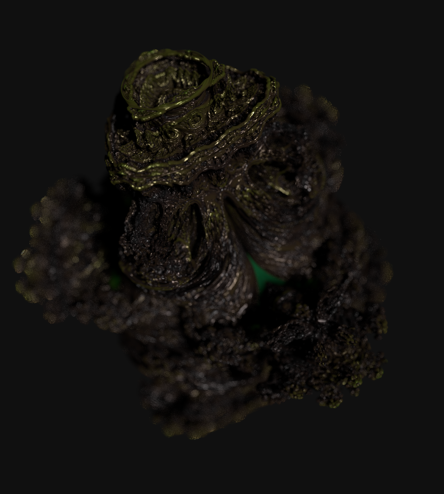
Shading
Now that we’ve covered all the separate components that are involved, we’ll put it all together and explain how points on the surface of the fractal are shaded. This is where the surface appearance comes to life: normals, shadows, materials, Fresnel, and BRDF terms all combine to decide the final pixel color.
Build the local shading frame
We start by constructing the vectors needed for lighting: the surface normal, view direction, light direction, and the half-vector used by the microfacet model. We also compute the key dot products that will be reused later.
// Build local shading frame for BRDF evaluation
vec3 n = getNormal(p);         // Surface normal estimated from distance field
vec3 v = normalize(-rd);       // View vector: from surface toward the camera

// SDF normals can sometimes flip inside cavities; correct if pointing away
if (dot(n, v) < 0.0) n = -n;

vec3 l = normalize(lightDir);  // Light direction (assumed normalized)
vec3 h = normalize(v + l);     // Half-vector: bisects view and light vectors

// Precompute common cosine terms for BRDF
float NdotL = max(dot(n, l), 0.0); // Normal–light cosine
float NdotV = max(dot(n, v), 0.0); // Normal–view cosine
float NdotH = max(dot(n, h), 0.0); // Normal–half-vector cosine
float VdotH = max(dot(v, h), 0.0); // View–half-vector cosine
| Symbol | Meaning |
|---|---|
n | Surface normal, estimated from the distance field. |
v | View direction toward the camera. |
l | Light direction (normalized). |
h | Half-vector, the normalized bisector of v and l. |
Soft shadows
Next we cast a secondary ray toward the light to evaluate how much of it is occluded. This produces soft shadow penumbras rather than hard binary shadows.
// Small offset along normal to prevent self-shadowing acne
float shadowBias = 2.0 * EPS_H;

// Shadow factor in [0,1]: 0 = fully in shadow, 1 = fully lit
float sh = softShadow(p + n * shadowBias, l, 0.0, FAR_T, 64);

// Apply shadowing by scaling NdotL
NdotL *= sh;

// Early exit if no contribution (in shadow or facing away)
if (NdotL <= 0.0 || NdotV <= 0.0) {
    return vec4(col, 1.0);
}
Base color and orbit trap
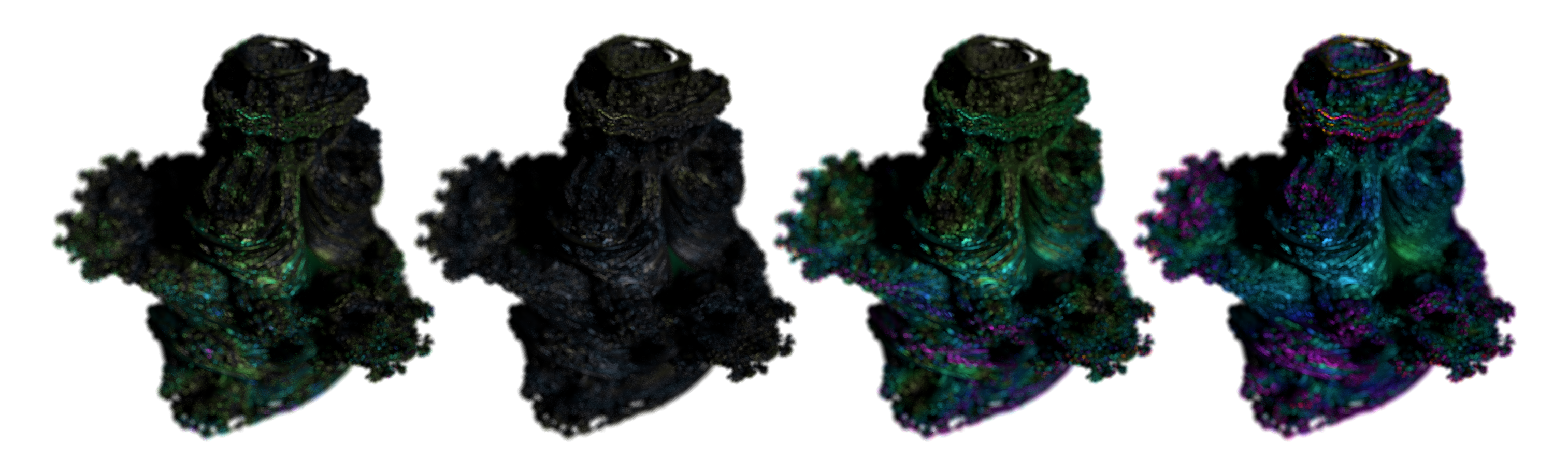
The base diffuse color comes from a uniform parameter. If orbit trap coloring is enabled, we blend it with a hue determined by the orbit trap value. This creates color variation that reflects the fractal’s internal geometry.
// Start with user-specified diffuse color
vec3 baseCol = diffuseColor;

// Optionally blend with orbit trap hue
if (useOrbitTrap) {
    vec3 hsvColor = hsv2rgb(vec3(trapVal, 1.0, 1.0));
    baseCol = mix(diffuseColor, hsvColor, trapVal);
}
Material parameters
Two main sliders control the look: metalness and roughness. Metalness decides whether the surface is a dielectric (like plastic) or a conductor (metal). Roughness controls how sharp or broad the highlights are.
// Clamp inputs to valid ranges
float m = clamp(metalness, 0.0, 1.0);  // Metalness: 0 = dielectric, 1 = metal
float r = clamp(roughness, 0.0, 1.0);  // Roughness: 0 = smooth, 1 = rough

// Convert perceptual roughness to microfacet slope variance
float alphaR = max(1e-3, r * r);
Cook–Torrance microfacet BRDF terms
We now calculate the terms of the Cook–Torrance microfacet BRDF:
| Term | Description |
|---|---|
F (Fresnel) | Controls how reflectivity increases at grazing angles. |
D (Distribution) | Shapes the highlight by describing how microfacets are oriented. |
G (Geometry) | Accounts for masking and shadowing of microfacets. |
// Base reflectance: 0.04 for dielectrics, base color for metals
vec3 F0 = mix(vec3(0.04), baseCol, m);

// Schlick Fresnel: angle-dependent reflectance
vec3 F  = fresnelSchlick(VdotH, F0);

// GGX normal distribution function
float D = (NdotH > 0.0) ? D_GGX(NdotH, alphaR) : 0.0;

// Smith geometry function with Schlick–GGX
float G = G_Smith_SchlickGGX(NdotV, NdotL, alphaR);
Specular reflection
The specular lobe is computed using the Cook–Torrance formula. This produces realistic highlights that become sharper when the surface is smooth and broader when it is rough.
// Cook–Torrance microfacet specular BRDF
vec3 specularBRDF = (D * G) * F / max(1e-4, 4.0 * NdotV * NdotL);

// Multiply by NdotL to account for light contribution
vec3 specular = specularBRDF * NdotL;
Diffuse reflection
Diffuse reflection is modeled as Lambertian, reduced by Fresnel (since some light is reflected specularly) and by metalness (since metals have little to no diffuse component).
// Diffuse energy balance
vec3 kD = (1.0 - F) * (1.0 - m);

// Lambertian BRDF
vec3 diffuse = kD * baseCol * (NdotL / PI);
Combine and debug override
Finally, we sum diffuse and specular terms to get the shaded color. There is also a debug toggle to visualize shadowing only, which helps inspect penumbra quality.
// Final shading: diffuse + specular
col = (diffuse + specular);

// Debug mode: visualize shadowed NdotL
if (uVisualizeShadows > 0.5) {
    col = vec3(NdotL);
}

return vec4(col, 1.0);
Progressive integration
Fractals with stochastic effects, anti-aliasing, soft shadows, and depth of field, look best when many slightly different samples are averaged together. Rather than firing thousands of rays in one expensive frame, this demo accumulates only a few samples per frame and progressively refines the image over a short window. This is how it works:
- Render the Mandelbulb once this frame into renderTarget.
- Full screen accumulation pass blends that result with the running average.
- Two floating point render targets (accumulationA and accumulationB) alternate as read and write targets (ping pong buffers):
tCurrentis this frame’s Mandelbulb rendertAccumis last frame’s average
- After compositing, the buffers swap:
[readTarget, writeTarget] = [writeTarget, readTarget].
All accumulation happens in linear (floating-point) targets; the final screen pass toggles encodeOutput = 1 to convert to display sRGB. Any parameter or camera tweak calls resetAccumulation() to reset state:
- Clears the accumulation targets
- Resets frameIndex to 1
- Restarts the integration window so we don’t mix incompatible samples.
Integration is timeboxed. The user can modify integrationTimeSec and bound how long accumulation lasts. When the timer elapses, the viewer simply re-displays the last refined frame until something changes.
This will help smooth noise from stochastic effects without tanking framerate. At the same time it maintains responsive interaction; we get a quick, coarse preview that sharpens in place. Finally we get deterministic convergence: the running average ensures stable results without bias.
On the big screen
In cinema, fractals are especially powerful because they create visuals that feel both organic and alien, infinite yet structured. Directors and visual effects teams often turn to fractals like the Mandelbulb to build surreal landscapes, impossible architectures, and otherworldly beings that would be difficult to design by hand. These structures lend a sense of depth and complexity that makes them perfect for science fiction, fantasy, and mind-bending visual storytelling.
- Infinite complexity & organic geometry: The Mandelbulb offers endlessly detailed and structurally rich visuals that are both mathematically precise and visually arresting.
- Alien and surreal resonance: Its uncanny, otherworldly look lends itself perfectly to sci-fi, fantasy, and mind-bending sequences.
- Flexible design motifs: Filmmakers and VFX artists use Mandelbulb geometry to evoke the ‘unknown’, whether in interdimensional portals, alien lifeforms, or futuristic landscapes.
Here are a few examples:
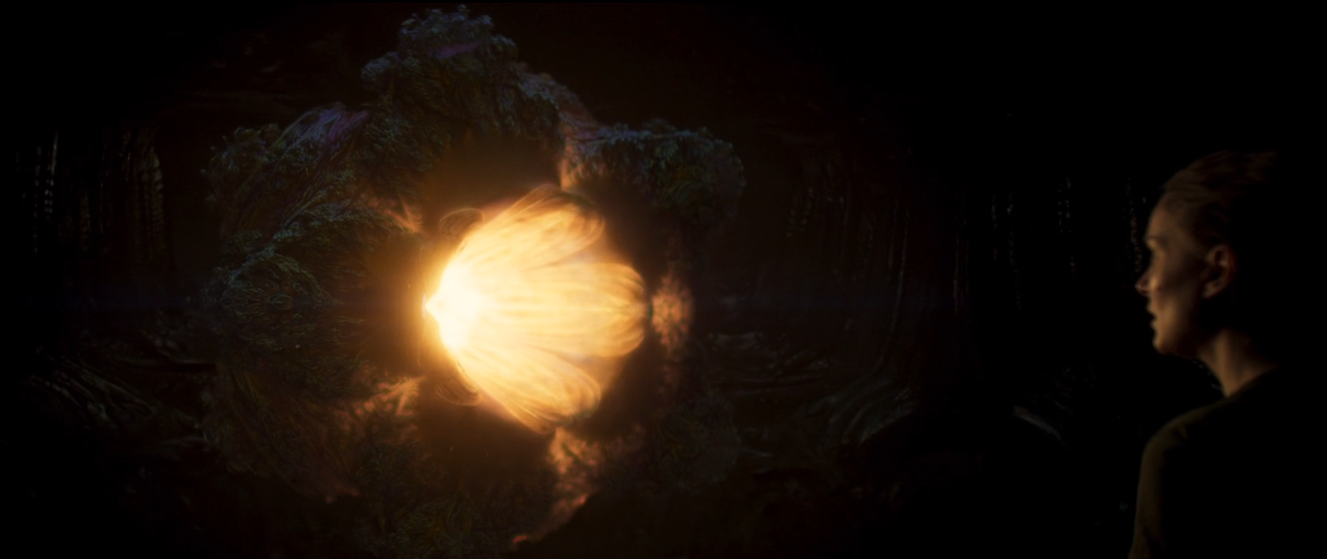
Annihilation (2018)
The climactic chamber and the alien entity itself are heavily inspired by Mandelbulb fractal geometry. The VFX team designed the alien’s form and the chamber set using Mandelbulb shapes generated in Houdini, even physically constructing elements of the set based on those shapes.
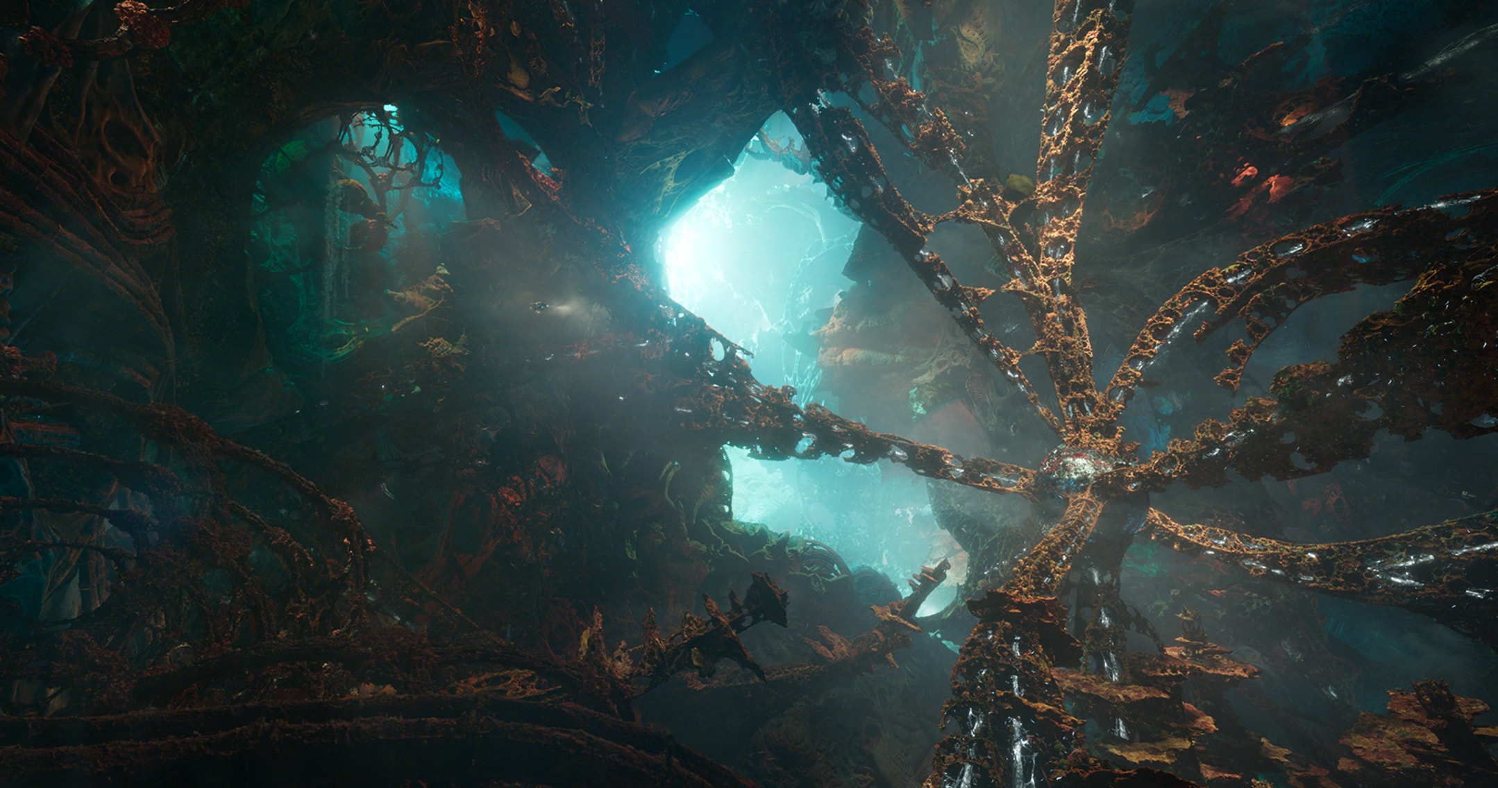
Big Hero 6 (2014)
In the film’s climax, Hiro and Baymax travel through a stylized wormhole whose interior resembles a swirling Mandelbulb structure; complex, organic, and fractal in nature.

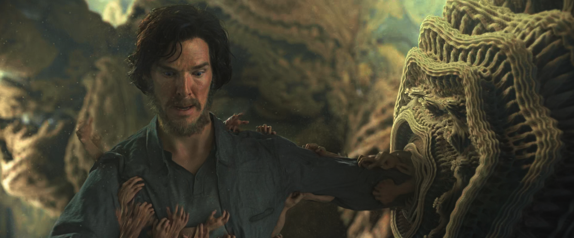
Doctor Strange (2016)
While exploring the metaphysical and “mirror” dimensions, the VFX team incorporated fractal inspired geometry, drawing heavily from the classic Mandelbrot set to suggest infinite, self-similar, reality-bending spaces.
Guardians of the Galaxy Vol. 2 (2017)
Hal Tenny, a visual artist using Mandelbulb 3D[03], contributed fractal based concept art for Ego’s palace and environment. The final VFX sequences incorporate these Mandelbulb inspired forms as architectural and landscape elements.
References / Further Reading
If you enjoyed this post or found the content helpful, I’d greatly appreciate your support! You can contribute via GitHub Sponsors to help me continue creating tutorials, demos, and open-source experiments. Every contribution, no matter the size, makes a difference and helps keep projects like this alive. Thank you!