Convolution
In mathematics, convolution is a binary operation over two functions. It is a fundamental concept in signal processing theory and has numerous applications in a variety of different fields, including image processing and optics. The operator is defined as:
\[(f * g) = \int_{-\infty}^{+\infty} f(\tau)g(t - \tau) dx\]Convolution is a commutative operator which provides a way of describing a Linear Time-Invariant (LTI) system by a signal g() and then compute the response to any signal f() by using the above formula. You are not required to understand the mathematics behind convolution to follow the rest of this post. However, if you would like to know more about it, watch the following MIT lecture from Dennis Freeman (Signals and Systems, Fall 2011).
Sobel Operator
The Sobel operator uses two 3×3 kernels which are convolved with the original image to calculate approximations of the derivatives [2] . One kernel is used for horizontal changes and one for vertical changes.
| \(A\) | Source Image |
| \(G_x\) | Horizontal derivative approximation |
| \(G_y\) | Vertical derivative approximation |
where
\(K_h\) is the horizontal kernel:
| +1 | +0 | -1 |
| +2 | +0 | -2 |
| +1 | +0 | -1 |
\(K_v\) is the vertical kernel:
| +1 | +2 | +1 |
| +0 | +0 | +0 |
| -1 | -2 | -1 |
The two derivatives are combined to compute the total gradient magnitude in the following way:
\[G = \sqrt{G_x ^ 2 + G_y ^ 2}\]Why does it work?
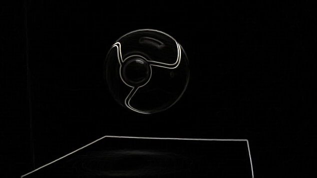
The resulting image consists of the edges of the objects that were depicted in the original image. This actually makes a lot of sense as the derivatives will by definition calculate the rate of pixel value change across the pixel grid. The edges seen in the final image are where there is a sharp color change in the original image, or in other words where the gradient magnitude has a high value. Finally it is worth noting that this method works better in lossless compression image formats, mainly because lossy compression algorithms tend to produce sharp artifacts in the resulting image.
Implementation
Below is an example implementation in a GLSL fragment shader. Note that the function that is used to combine the derivatives is scaled to control the intensity of the effect.
uniform sampler2D iChannel0;
uniform vec3 iResolution;

vec3 sample(const int x, const int y)
{
    vec2 uv = (gl_FragCoord.xy + vec2(x, y)) / iResolution.xy;
    return texture2D(iChannel0, uv).xyz;
}

float luminance(vec3 c)
{
    return dot(c, vec3(0.2126, 0.7152, 0.0722));
}

vec3 edge(void)
{
    vec3 hc = sample(-1,-1) *  1.0 + sample( 0,-1) *  2.0
            + sample( 1,-1) *  1.0 + sample(-1, 1) * -1.0
            + sample( 0, 1) * -2.0 + sample( 1, 1) * -1.0;
    vec3 vc = sample(-1,-1) *  1.0 + sample(-1, 0) *  2.0
            + sample(-1, 1) *  1.0 + sample( 1,-1) * -1.0
            + sample( 1, 0) * -2.0 + sample( 1, 1) * -1.0;

    return sample(0, 0) * pow(luminance(vc*vc + hc*hc), 0.6);
}

void main(void)
{
    gl_FragColor = vec4(edge(), 1.0);
}
Here’s a live preview and captures of the shader in action:

