Distance Culling
The scene objects are culled depending on their distance from the camera. If they are further than their maximum drawing distance or closer than their minimum drawing distance they are not drawn.
Frustum Culling
The view frustum is defined by the projection and represents a volume of space that the camera can see. In the case of 3D perspective projection the view frustum has a trapezoidal shape. All polygons are clipped against the frustum during rasterization and therefore geometry that is not within the bounds of the frustum will not be visible on screen. In order to avoid extraneous calculations , an early rejection strategy must be adopted. The simplest implementation would involve using a bounding volume for each object of the scene in order to quickly test against the frustum for occlusion. Spheres are commonly used due to the low computational cost. A sphere is out of the frustum if its center is on the wrong side of at least one plane and the distance to that plane is greater than the radius of the sphere. If the absolute value of the distance is smaller than the radius then the sphere intersects the plane, meaning that the sphere is partially within the frustum.
This method is a rough approximation and is usually employed as a first pass to quickly reject large chunks of geometry. Partially occluded objects would still be rendered and subsequently clipped against the frustum even if very few or none of the object’s polygons are within the frustum.
Backface Culling
In most cases it is better to avoid rendering polygons that are not oriented towards the camera. One method of implementing backface culling is by discarding all triangles for which the dot product of their surface normal and the camera view vector is equal to or greater than zero.
Early Z Rejection
Starting with the GeForce3 GPU, all NVIDIA GPUs (and many from other vendors) support early-z rejection. In the rasterizer stage of the rendering process, early-z compares the depth value of a fragment to be rendered against the value currently stored in the z-buffer. If the fragment is not visible (because the depth test failed), rejection occurs without fetching the texture for the fragment or executing the fragment program. The result: memory bandwidth is saved at the per-fragment level. This approach re quires to manually sort the objects from front to back. As the depth buffer and the stencil buffer are often stored together, using the stencil buffer may reduce early-z performance.
GPU Occlusion Queries
In OpenGL, the ARB_occlusion_query extension (which is based on NVIDIA’s NV_occlusion_query extension, a much-improved form of Hewlett-Packard’s original HP_occlusion_test extension) implements the occlusion query idea on the GPU and fetches the query results.
Microsoft has incorporated the same functionality in DirectX 9. The main idea behind a query is that the GPU reports how many pixels should have ended up visible on-screen. These pixels successfully passed various tests at the end of the pipeline - such as the frustum visibility test, the scissor test, the alpha test, the stencil test, and the depth test. Similarly to early z rejection, the objects must be manually sorted from front to back in advance in order to achieve any level of efficiency.
The process is summarized as follows:
- Create n queries.
- Disable rendering to screen.
- Disable writing to depth buffer.
- For each of n queries:
- Issue query begin.
- Render the object’s bounding box.
- End query.
- Enable rendering to screen.
- Enable depth writing (if required).
- For each of n queries:
- Get the query result.
- If the number of visible pixels is greater than 0, render the complete object.
These steps allow substituting a geometrically complex object with a simple bounding box. This bounding box will determine whether the object neeeds to be rendered. If the object’s bounding box ends up occluded by other on-screen polygons, it can be skipped entirely. It is worth mentioning that multiple outstanding queries are possible.
There are caveats to the method, more specifically using bounding boxes in the query step might lead to incorrect results as depicted below:

A way to fix this involves delaying the queries by a frame and rearranging the steps, however that introduces a different set of problems. Another approach would be to use a carefully constructed LOD instead of using a bounding box.
Coherent Hierarchical Culling
This method optimizes the use of GPU Occlusion Queries by considering temporal and spatial coherence of visibility.
BSP with Potential Visible Sets (PVS)
BSP stands for Binary Space Partitioning. In Binary Space Partitioning, space is split with a plane to two half spaces, which are again recursively split. This can be used to force a strict back to front drawing ordering. Occlusion culling in BSP based engines is usually based on the Potentially Visible Set (PVS). This means that, for every cell in the world, the engine finds all the other cells that are potentially visible from the cell, from any point in the cell. At render time, the cell where the viewer is located is found, view frustum culling is performed for the cells in the PVS, and finally those cells that reside in the PVS and inside the frustum are drawn. This introduces several major concepts . PVS-based culling is conservative in the sense that it always overestimates the set of visible cells. This means that no artifacts should ever occur due to visible objects not being drawn. Calculating the PVS is an expensive offline process that is traded for the ability to do fast queries at runtime.
The main problem with PVSs is the high level of overdraw, meaning that a lot of redundant polygons are typically drawn; this is due to the fact that a PVS contains all the cells that can be seen from anywhere in the viewing cell. The overdraw typically ranges from 50% to 150%. There are a lot of derivative methods that attempt to reduce the overdraw level.
Portals
This is a cell based occlusion culling method and as such it relies on the assumption that the game world can be divided to cells that are connected to each other. A portal is a n-sided flat convex polygon, handled in a special way at rendering time. It is not renderable and it is used to define an area that can be crossed to go from one section to another in the level (eg. a door between two rooms, a window, a hole in a wall…).
If a portal is visible by the camera this means that the camera can potentially see what is on the other side of the portal. A portal establishes a link between two graph nodes that don’t necessarily have any other relationship. The rendering of the scene doesn’t start at the scene graph’s root, but at the node in which the camera is located (a simple SP structure like an octree can be used to determine this). This node’s sub tree is rendered and then visibility of the portals is determined. A variety of different methods can be used at this stage. An engine that combines precalculated portal graphs for static geometry with another method for dynamic objects could employ CPU based hierarchical z buffer testing at this stage to quickly determine if the portals are visible, while an engine with a simpler architecture could use a less effective method such as frustum culling. For each visible portal the connected node is rendered using the same procedure recursively. Portals can be very useful for static interior scenes but would not be effective in the case of dynamic destructible geometry (eg. physics based destructible walls) or massive exterior environments.It should be noted that portals can be connected in a loop and this can lead to infinite recursion loops therefore mechanisms must be in place to deal with that problem.
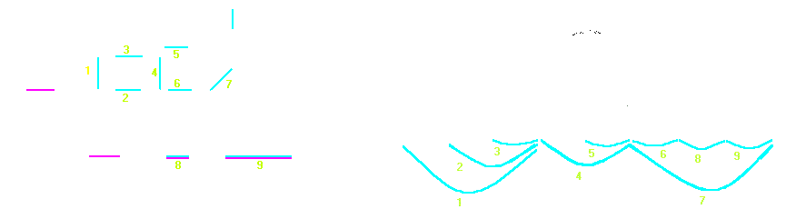
In the diagram below the blue lines define an association between two rooms by means of a portal (numbers in green).
Anti-Portals
This is, as the name suggests, the exact opposite of portals.
Hierarchical Z-Buffer Occlusion Culling
The main idea behind this method is to render a simplified version of all the geometry to a z-buffer and use mipmaps of the depth buffer to determine visibility, minimizing the number of tests required per object. The process can be broken down to the following steps:
- Determine a set of potentially visible occluders with frustum culling. (Bounding spheres or Bounding Boxes can be used in this step.)
- Render the occlusion volumes of the remaining objects to a small render target with a full mip chain. The occlusion volumes can be handmade CSGs made out of cubes or precalculated voxel based procedural approximations of the original geometry. It is very important that each occlusion volume is restricted to the internal area of the corresponding model and does not go beyond its bounds.
- Conservatively downsample the depth buffer into the other levels of the mip chain. This will produce conservative depth buffers with a coarser approximation at each subsequent level.
- For each object, render and determine the maximum screen space width and height of the bounding box and then use that to calculate the mip level to sample from so that the object does not cover more than a 2-pixel square region (4 samples in total).
- If the maximum sampled depth value is closer than the closest depth value for the object then the it’s completely occluded.
- Use a writable buffer to store a visibility flag (float value of 0. or 1.) for each object so that this information can be copied across and later on accessed by the CPU. For a more detailed description of the method along with code samples please refer to
The Umbra 3 Method
Umbra uses a custom world editor that processes the static world geometry as a polygon soup, voxelizes and subdivides the scene into view cells and generates a portal graph and cell potentially visible sets (PVS) for the entire scene. The exported data is store in a database called the Tome which is used at runtime to perform camera and region queries on the client side via the Umbra API. To account for dynamic geometry, the visibility queries can provide a conservative depth buffer (with the use of a in-house rasterizer) against which dynamic occluders can be tested quickly.