Distributed ray-tracing is a term that is commonly misconstrued, and often associated with the concept of parallel computing, where the calculations required to render an image are distributed across a network of processing nodes. The more appropriate term, ‘parallel ray-tracing’ is typically used to resolve the ambiguity.
Whitted Ray-Tracing
In the traditional Whitted algorithm, a ray is spawned, for every pixel in the screen. That ray is tested against the geometry of the scene to check whether an intersection point exists. If an intersection is found, depending on the properties of the surface, a limited number of additional purpose specific rays may be generated.
These rays can either be shadowing rays, that check whether the resolved point is visible or not by the light sources in the scene, or reflection / transmission rays that recursively trace a specular light path to model reflection or transmission events in perfect mirrors and transparent media.
While the algorithm can produce aesthetically pleasing results and is able to model interactions that traditional rasterization fails to represent at the same level of visual fidelity, it can only simulate a limited set of interactions and light paths, most of which are not typically observed in the real world. In a mathematical sense, it’s intuitive to think of the limitations in terms of the rendering equation which requires the evaluation of several integrals. Conventional ray-tracing is estimating illumination using a single sample across the entire domain, which constitutes a particularly crude approximation.
In summary some of the limitations are:
- Shadows have a hard edge, as only infinitesimally small point light sources of zero volume can be simulated, with binary shadow queries that use a single ray.
- Reflection / Refraction can only simulate a limited set of light paths, for perfect mirror surfaces, or perfectly homogeneous transparent media.
- More complex effects like depth of field are not supported.
Distributed Ray-Tracing
Distributed ray-tracing, also known as ‘stohastic ray-tracing’, takes a few additional steps towards photo-realism, adding support for simulating smoothly varying optical phenomena.
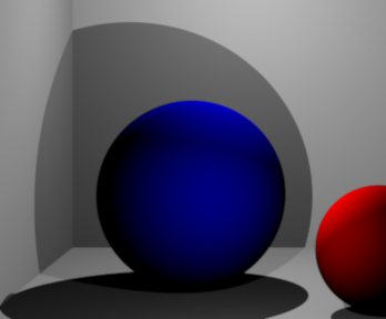
To simulate light sources of arbitrary size and shape, shadowing queries are required to yield non binary results. In the real world, a light emitter can be visible in it’s entirety, partially occluded or fully occluded at a specific point on a surface. The resulting shadow has a characteristic gradient border, that is typically called the shadow’s ‘penumbra’. Distributed ray-tracing simulates this effect, by adopting a probabilistic approach. A random point on the light emitter’s surface is selected at random and a shadow ray is constructed, originating from the point that is being shaded, towards that randomly picked position. Multiple such samples are integrated to approximate the occlusion probability for the shaded point.
The same approach is used to simulate a variety of interactions and optical effects:
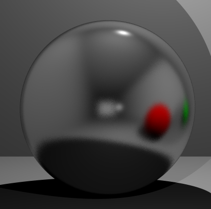
- Different degrees of glossiness can be simulated by generating multiple reflection rays towards random samples on a specular lobe.
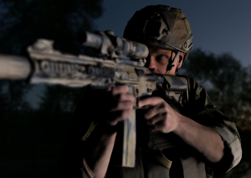
- Optical depth of field is computed by distributing multiple integration samples on a thin lens geometry.
- Motion blur can be achieved by integrating multiple samples in the time domain.
Looking at the rendering equation once again, it’s easy to see that the Monte Carlo method used in distributed ray-tracing, samples the integrand at multiple points across the domain, averaging the result to calculate a far better approximation.
Samples
Below you can find some examples that I generated using my own renderer: xtracer. The project is open source and you can access the code Github.


Example Code
Here is an example on how to implement the thin lens model shown above. The full source is available in Github
Ray Perspective::get_primary_ray(float x, float y, float width, float height)
{
  // Note that the direction vector of ray is not normalized.
  // The DoF ray calculation depends on this at the moment.
  Ray ray;

  scalar_t aspect_ratio = (scalar_t)width / (scalar_t)height;
  ray.origin = position;

	// Calculate the ray's intersection point on the projection plane.
	ray.direction.x = (2.0 * (scalar_t)x / (scalar_t)width) - 1.0;
	ray.direction.y = ((2.0 * (scalar_t)y / (scalar_t)height) - 1.0) / aspect_ratio;
	ray.direction.z = 1.0 / tan(fov * RADIAN / 2.0);

	/*
		Setting up the look-at matrix is easy when you consider that a matrix
		is basically a rotated unit cube formed by three vectors (the 3x3 part) at a
		particular position (the 1x3 part).

		We already have one of the three vectors:
			-	The z-axis of the matrix is simply the view direction.
			-	The x-axis of the matrix is a bit tricky: if the camera is not tilted,
				then the x-axis of the matrix is perpendicular to the z-axis and
				the vector (0, 1, 0).
			-	The y-axis is perpendicular to the other two, so we simply calculate
				the cross product of the x-axis and the z-axis to obtain the y-axis.
				Note that the y-axis is calculated using the reversed z-axis. The
				image will be upside down without this adjustment.
	*/

	// Calculate the camera direction vector and normalize it.
  calculate_transform(m_transform);

	// Calculate the deviated ray direction for DoF
  if (flength > 0) {
      Ray fray;
    fray.origin = ray.direction;
    scalar_t half_aperture = aperture / 2.f;
    fray.origin.x += prng_c(-half_aperture, half_aperture);
    fray.origin.y += prng_c(-half_aperture, half_aperture);

      // Find the intersection point on the focal plane
    Vector3f fpip = ray.direction + flength * ray.direction.normalized();
    fray.direction = fpip - fray.origin;

      ray = fray;
  }

	// Transform the direction vector
	ray.direction.transform(m_transform);
	ray.direction.normalize();

	// Transform the origin of the ray for DoF
  if (flength > 0) {
    ray.origin.transform(m_transform);
    ray.origin += position;
  }

	return ray;
}

